Create a Wine Recommender Using NLP on AWS
Use AWS SageMaker to create sentence-BERT embeddings and run realtime Nearest Neighbors inferences
Getting Started
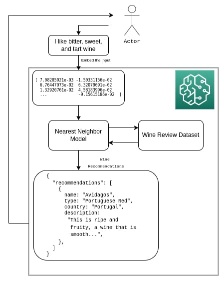
In this tutorial, we’ll build a simple machine learning pipeline using a BERT word embedding model and the Nearest Neighbor algorithm to recommend wines based on user inputted preferences. To create and power this recommendation engine, we’ll leverage AWS’s SageMaker platform, which provides a fully managed way for us to train and deploy our service.
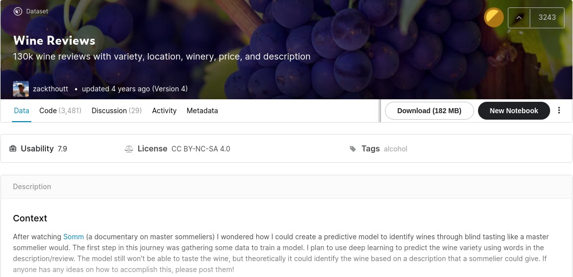
The dataset we'll use includes more than 130,000 different wines and corresponding reviews. We'll use BERT to convert the wine reviews into embeddings (i.e. vectors) and store those embeddings in AWS S3. We’ll then use that as our dataset for the Nearest Neighbor search, which will then be able to accept new user input, create an embedding for it, and find the K closest embeddings to that user input. The ultimate outcome Identifying and recommending wines with reviews most similar to the input the user provided.

Note: This tutorial is set up in a way where you should have a working version if you program along, though we’ll skip trivialities such as installing dependencies and importing packages. If you’d like to follow along with the code, make sure to have an AWS S3 bucket you can use to store the dataset and a SageMaker Notebook in the same region with permissions to access that S3 bucket (see example IAM policy below). If you’d rather just skip to the end and run the final working version, you can find the full Jupyter Notebook and Python scripts in this tutorial’s Github page.
{
    "Version": "2012-10-17",
    "Statement": [
        {
            "Sid": "VisualEditor1",
            "Effect": "Allow",
            "Action": "s3:*",
            "Resource": "arn:aws:s3:::<bucketName>/*"
        }
    ]
}
Data Collection
With our fresh S3 bucket and SageMaker notebook created, we should first create some global variables that other cells in our notebook can use.
role = get_execution_role()
bucket = "<S3_BUCKET>"
prefix = "<S3_KEY_PREFIX>"
filename = "<DATASET_FILENAME>"
raw_data_location = f"s3://{bucket}/{prefix}raw/{filename}"
This specifies two things:
- The S3 buckets and prefixes that you want to use for saving model data and where training data is located. These should be within the same region as the Notebook Instance, training, and hosting.
- The IAM role ARN used to give SageMaker access to your data. It can be fetched using the
get_execution_role()method from SageMaker Python SDK.
This defines everything we’ll need to upload our dataset to the S3 bucket. The dataset we’re using isn’t included in an ML framework like MNIST, so we’ll need to pull it directly from Kaggle. The opendatasets library can assist us with that and boto3 can be used to upload the dataset to S3.
od.download("https://www.kaggle.com/zynicide/wine-reviews")
inputs = boto3.resource("s3").Bucket(bucket).upload_file(
    f"wine-reviews/{filename}", f"{prefix}raw/{filename}"
)
Note: this requires a Kaggle account and access token. If you don’t have a Kaggle account or don’t want to make one, you can download the dataset directly from the website and upload it to S3 using the AWS console. Just make sure that if you’re doing it this way, you store it with the correct prefix or things will break later.

To verify that everything is set up for the next steps, you can read in the dataset using df=pd.read_csv(raw_data_location) and then run things like
df.describe() or df.head(5). This’ll also give you a good look at how the data is structured and what fields it contains.
Data Preprocessing
When training large models with huge amounts of data, you'd typically use big data tools like Amazon Athena, AWS Glue, or Amazon EMR to extract, transform, and load data to and from S3. Fortunately, we aren't using too much data so we can use the tools provided by the SageMaker Python SDK and pandas to clean and upload the data to our bucket.
Although BERT is fully capable of taking in our wine descriptions as-is with no modifications needed, there are several steps we can take to preprocess our data to achieve better results. This tutorial’s purpose may be mostly educational so accuracy isn’t necessarily a major concern, though it’s still good practice to always preprocess your data before feeding it into a model.
The preprocessing steps we’ll take for our data are:
- Lowercase every character
- Remove punctuations
- Lemmatize the words
- Specifically using english lemmatization techniques
def clean_data(desc):
    words = stopwords.words('english')
    lower = " ".join([w for w in desc.lower().split() if not w in words])
    punct = ''.join(ch for ch in lower if ch not in punctuation)
    wordnet_lemmatizer = WordNetLemmatizer()

    word_tokens = nltk.word_tokenize(punct)
    lemmatized_word = [wordnet_lemmatizer.lemmatize(word) for word in word_tokens]

    word_joined = " ".join(lemmatized_word)

    return word_joined
This code is written inside a function on purpose because with it packaged as a function, we can apply it to every row in the dataframe:
df['clean_desc'] = df["description"].apply(clean_data)
To see what our new, cleaned descriptions look like, feel free so run something like df['clean_desc'].head(5). If everything looks right, we can go ahead and upload our new cleaned dataset to S3. This will put us in a good place to finally use BERT to generate embeddings.
# Upload the preprocessed dataset to S3
df.to_csv("dataset.csv")
clean_data_location = f"{prefix}clean/dataset.csv"
inputs = boto3.resource("s3").Bucket(bucket).upload_file('dataset.csv', clean_data_location)
Generate Embeddings
Since BERT is a pretrained model, But while no explicit training is needed, it’s useful to think of the embeddings generation as a “training” step. By doing this, we can use all the tools SageMaker providers to train models and use them to generate our embeddings (with a little bit of finessing, of course).
The SageMaker way of setting up a training job is to use an Estimator. This Estimator is an object that’ll contain information about our Python version, framework version, hyperparameters, the instance type we want to use, how to explicitly train the model, etc. It’s a powerful tool. The Estimator expects the training instructions to be in a Python script (which you can find in the Github repo).
In our case, the training script uses a library called sentence-tranformers to drive BERT and the library uses PyTorch under the hood. For this reason, we’ll be creating a PyTorch Estimator,which is essentially a generic Estimator with some extra PyTorch libraries and tools installed on it.
embeddings_estimator = PyTorch(
    role = role,                          # Our AWS role
    entry_point ='embeddings_script.py',  # The training script
    instance_type="ml.m5.large",          # The ec2 type
    instance_count=1,                     # Number of ec2
    source_dir = './src',                 # The source directory
    framework_version = '1.9.0',          # PyTorch version
    py_version = 'py38',                  # Python version
    sagemaker_session=sagemaker.Session(),

        # Where to put the embeddings
    output_path=f"s3://{bucket}/model/embeddings",

        # Model hyperparameters
    hyperparameters={
        'output-data-dir': "/opt/ml/output/data/",
        "embeddings-output-path": f"s3://{bucket}/model/embeddings/embeddings.csv.tar.gz",
    },
)
Creating the Estimator won’t create our model, it’ll just store metadata for it. To actually train and get our model, we’ll need to run fit() on it, which expects an S3 location to our training data. Another important by-product of this is not only our embeddings, but also a model to generate new embedding based on input we’ll receive in the future.
embeddings_estimator.fit({
    'train': f"s3://{bucket}/{prefix}clean/dataset.csv"
})
print("[+] finished model fitting")
Running this will take a while depending on the instance_type and for us, it took about an hour.
Behind the scenes, defined in the Python script, SageMaker is generating our embeddings inside a PyTorch Docker container running on a machine
learning-optimized EC2 instance. Once the model is done being fitted, the embeddings should be stored in S3 in the location we supplied to the Estimator. To verify that it actually worked, we can create a Predictor object. We do this using the deploy() method which’ll deploy our model on AWS as a SageMaker Endpoint.
timestamp_prefix = strftime("%Y-%m-%d-%H-%M-%S", gmtime())
embeddings_endpoint_name = "embeddings-model-ep-" + timestamp_prefix

embedding_predictor = embeddings_estimator.deploy(
    instance_type='ml.m5.large',
    initial_instance_count=1,
    endpoint_name=embeddings_endpoint_name,
    serializer=JSONSerializer(),
    deserializer=JSONDeserializer(),
)
This endpoint can be pinged from our notebook and gives us a way of verifying that our embedding model is doing its job correctly.
test_embedding = embedding_predictor.predict(
    {"data": "sweet wine with a hint of tartness"}
)
print(len(test_embedding["embeddings"]))
Nearest Neighbors
Now we need to repeat that model creation process for our Nearest Neighbor model. This’ll be very similar to one before in that we’ll create a Sagemaker Estimator object.This time, it’ll be a SKLearn Estimator, which’ll store our training and inference metadata, and we’ll run fit() on it to train and build our model.
nn_estimator = SKLearn(
    entry_point='nn_script.py',
    source_dir = './src',
    instance_type="ml.m5.large",
    instance_count=1,
    role=role,
    sagemaker_session=sagemaker.Session(),
    framework_version="0.23-1",
    py_version="py3",
    hyperparameters={
        'n_neighbors': 10,
        'metric': 'cosine',
    },
)
The training data for Nearest Neighbor is the embeddings we generated in the previous section.
nn_estimator.fit({
    'train': f"s3://{bucket}/model/embeddings/embeddings.csv.tar.gz"
})
Again, similar to the previous model, we can test that everything is working correctly by deploying the Nearest Neighbor model and sending it random input.
timestamp_prefix = strftime("%Y-%m-%d-%H-%M-%S", gmtime())
nn_endpoint_name = "nn-model-ep-" + timestamp_prefix
nn_predictor = nn_estimator.deploy(
    instance_type="ml.m5.large",
    initial_instance_count=1,
    endpoint_name=nn_endpoint_name,
)
predictor = Predictor(
    endpoint_name=nn_endpoint_name,
    sagemaker_session=sagemaker.Session(),
    serializer=JSONSerializer(),
    deserializer=JSONDeserializer(),
)

test = test_embedding["embeddings"]

prediction = predictor.predict(
    {"embeddings": test, "kneighbors": 5}
)
print(prediction['recommendations'])
Inference Pipeline
Now we have both the BERT model created for embeddings and the Nearest Neighbor model for making recommendations. The only question left is: how do we connect the two?
Connecting them with a lambda could work, but it would be slow, complicated, and require a lot of network traffic between lambda and SageMaker (not to mention the lambda would likely timeout on some requests). Luckily, SageMaker has a very nice and idiomatic way of connecting several models together, called an InferencePipeline.
timestamp_prefix = strftime("%Y-%m-%d-%H-%M-%S", gmtime())
endpoint_name = "inference-pipeline-ep-" + timestamp_prefix
pipeline_model = PipelineModel(
    role=role,
    models=[
        embeddings_estimator.create_model(),
        nn_estimator.create_model(),
    ],
    sagemaker_session=sagemaker.Session(),
)
inference_pipeline = pipeline_model.deploy(
    initial_instance_count=1,
    instance_type="ml.m4.xlarge",
    endpoint_name=endpoint_name,
    serializer=JSONSerializer(),
    deserializer=JSONDeserializer(),
)
pipeline_predictor = Predictor(
    endpoint_name=endpoint_name,
    sagemaker_session=sagemaker.Session(),
    serializer=JSONSerializer(),
    deserializer=JSONDeserializer(),
)
We’ll make our request with the payload in 'application/json' format, since that is what our script currently supports. If other formats need to be supported, this would have to be added to the output_fn() method in our entry point. The prediction output in this case is trying to guess the wines with the most similar reviews to the one inputted.
test_payload = {"data": "sweet wine with a hint of tartness"}
test_response = pipeline_predictor.predict(data=test_payload)

print(test_response)

Clean Up
Finally, we should delete the model and endpoint before we close the notebook (unless you really wanted the wine recommender to be always available).
# Delete endpoint and endpoint configuration
embedding_predictor.delete_predictor()
nn_predictor.delete_predictor()
pipeline_predictor.delete_predictor()
In case you’ve run model creation steps multiple times, the following will only remove the most recent, so you will need to manually remove all other versions of the models and endpoints.
Next Steps & Improvements
With AWS SageMaker we’ve created a highly scalable machine learning pipeline, but we’re limiting ourselves a little bit by just using a single CSV file as our database. Replacing this with an actual database or piping the data in from a Data Lake on the backend could potentially improve performance and, at a minimum, allows us to further scale to larger datasets.
Experimentation with different models could potentially improve accuracy. For instance, an algorithm like TF-IDF may be better suited for this type of search. We saved a bit of development time by using a pre-trained BERT model, but fine tuning of embeddings models on related datasets has been shown to greatly improve accuracy in other pipelines, as mentioned in this article as well as many others, this would probably greatly improve the quality and accuracy of our results.
Check out the full source code for the project, including the Jupyter Notebook. For further reading on some of the topics discussed in this post, take a look at the following resources.
- Link to the dataset on Kaggle
- How to fine-tune sentence-BERT
- Hugging Face
- A list of other sentence transformers
- Official BERT paper
- BERT wiki
- More SageMaker tutorials (NLU item search)
- More SageMaker examples (Text item search)
- A wine recommender blog series
Cover Photo by Abby Dohmeier

